Robotics Control Research Lab
I worked as a research assistant for Dr. Aykut Satici in his robotics control lab at Boise State. The lab is teaching a neural network to do dynamic, contact-rich manipulation: an actor-critic controller written in Python commands the forces and torques that drive a robot arm, and it has to learn to push a box up onto a step and park it at a target pose without any of the contact behaviour being hand-scripted.
My own work centered on two things: hunting down bugs in the training pipeline, and building the export path that takes a trained controller out of Python so it can run on real hardware.
Finding the loss function bug
When evaluating a controller, the loss was being computed for every trial in a batch and then summed into a single scalar, so an entire batch of runs collapsed into one number. The symptom that gave it away was that evaluation runs from a given starting pose kept producing suspiciously similar losses no matter what the controller actually did. Once that was fixed we could finally see per-run behaviour, which is what let the team start genuinely debugging the controller instead of guessing at aggregate numbers.
The gap function
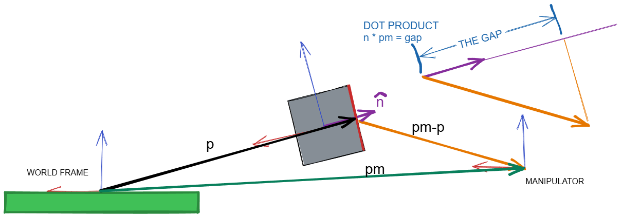
The gap function returns the perpendicular distance from the manipulator to each of the box's four faces, and the loss uses those distances to encourage the controller to stay in contact with the correct face. It is central to the whole reward structure, and it was subtly wrong, so another student and I sat down and mapped out the geometry from scratch — building the outward face normals from the box's rotation matrix and taking dot products against the vector from the face to the manipulator. The diagram below is the one we drew to reason about it. Working it out on paper first is what made the bug findable in the code.
From there I worked with him on trying different loss functions and training new controllers to see what the changes actually bought us.
Exporting controllers to real hardware
A trained controller lived as an Equinox .eqx file, which is only useful
inside Python and JAX. To run one on a real robot it needs to be callable from C++, so I built a pipeline that
exports a trained controller to ONNX, verifies it, and benchmarks it.
This took a lot of trial and tribulation, but eventually, the thing that worked was
using the jax2onnx library, which converts straight from the Equinox module. It pins
a JAX version incompatible with the rest of the project, so the exporter runs inside its own throwaway virtual
environment that the shell wrapper builds from a pinned requirements list. In other words, I spend weeks
fighting dependencies until I was able to get the thing to work.
After conversion it runs random state vectors through both the ONNX model and the original Equinox controller and asserts they agree to within 1e-6, then benchmarks inference in Python and again in C++. If any check fails it deletes the partial output and exits nonzero, so a subtly broken controller can never end up sitting on disk looking valid. Inference came out around 40 kHz in Python and 60 kHz in C++, far more than robot control needs. A useful side effect is reproducibility: an ONNX file freezes the traced computation graph, so a controller stays runnable even after the training code has moved on underneath it.
What I took away from it
This was my first experience of real research, and of working in a large, genuinely technical codebase that I did not write and could not hold entirely in my head. It was also cross-team: our lab at Boise State worked alongside a different group at the University of Kentucky that focused on the real hardware aspect of things.
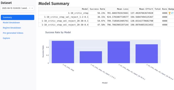
A friend and fellow student worked in the lab alongside me, and the thing that made us productive was being honest about what each of us was better at and splitting the work along those lines instead of both half-doing everything. He built the evaluation dashboard, which I then used constantly to judge whether a controller I had trained was actually an improvement; I took the export pipeline and a lot of the bug hunting. Where the work genuinely needed both of us, like untangling the gap function, we sat down and did it together. Delegating to our respective strengths made us meaningfully faster than working in parallel on the same things would have.
A Perfect Run
A controller I trained, solving the task from the hardest starting position: the manipulator pushes the box up onto the step and settles it on top. This is a cherry picked success, but it demonstrates what the models are capable of.
Gap Function Diagram
The diagram another student and I drew to work out how the gap function computes the distance from the manipulator to a face of the box: the face normal dotted with the vector from the face to the manipulator. Mapping it out this way is what let us debug it.
The Simulated Environment
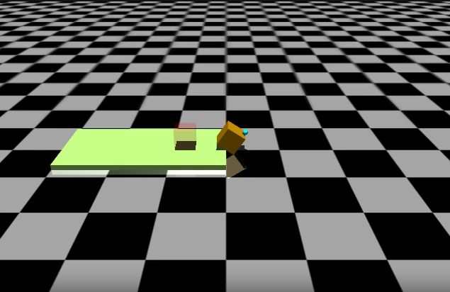
The MuJoCo scene the controller is trained in: the manipulator, the box it has to move, and the step it has to get the box onto.
Evaluation Dashboard
The dashboard my fellow student built over our batch evaluation results, which I used to compare controllers. Each model is run through many episodes across several starting-condition regimes, and the dashboard summarizes success rate, mean loss and control effort, then lets you drill into individual trajectories and rendered videos.